SDE Sample Path
Chapter 18: Langevin Dynamics and Sampling — Diffusion Preview
From the book
Chapter 18: Langevin Dynamics and Sampling. In the chapter mind map this icon labels Diffusion Preview: Continuous-Time SDEs. The discussion below is excerpted and lightly edited from § Derivation from Continuous-Time Limit in Mathematics for AI and Machine Learning.
The discrete update can be derived by discretizing the continuous-time Langevin SDE:
Using the Euler-Maruyama discretization (see Chapter the referenced section) with time step $\eta$:
where $\boldsymbol\epsilon \sim \mathcal{N}(\mathbf{0}, I)$ and $\sqrt{\eta} d\mathbf{W}_t \approx \sqrt{\eta} \boldsymbol\epsilon$. Setting $\sqrt{2\eta} = \sqrt{2} \sqrt{\eta}$ gives the discrete update formula.
The factor $\sqrt{2}$ comes from the requirement that the stationary distribution of the continuous process matches the target distribution $p(\mathbf{x})$. This is a consequence of the fluctuation-dissipation theorem from statistical physics.
What this drawing shows
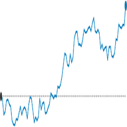
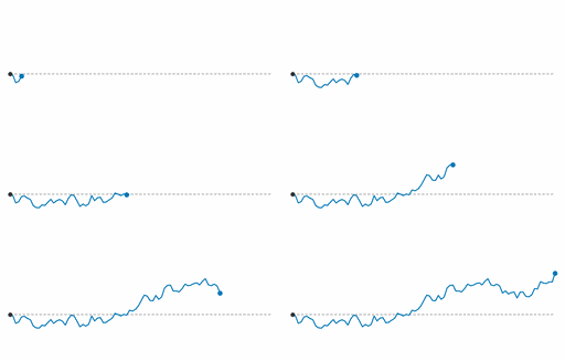
What you see. Brownian sample path fluctuates around dashed $\mathbb{E}[x_t]=0$; animation grows the noisy trajectory from $t{=}0$ to $T$.
In the mind map. Chapter 18 — Diffusion Preview: Continuous-Time SDEs. See From the book above for definitions, figures, and worked examples.
Where to read next
Read the full definitions, figures, and worked examples in Chapter 18: Langevin Dynamics and Sampling — see the mind-map node Diffusion Preview: Continuous-Time SDEs.